Week 11 - Ligand Binding, Docking and Drug Discovery
Molecular docking is a computational technique that predicts how a small molecule (ligand) binds to a target macromolecule (receptor) by exploring possible orientations and conformations, then scoring each pose by estimated binding affinity. It is a cornerstone of structure-based drug design (SBDD) — enabling researchers to screen millions of compounds in silico before committing to expensive synthesis and biological assays.
How Docking Works
- Receptor preparation — The target protein is cleaned, protonated, and assigned atomic partial charges.
- Ligand preparation — The drug candidate is converted to a 3D format with proper charges and a defined torsion tree (rotatable bonds).
- Search — The docking engine places the ligand inside a defined search space (grid box) on the receptor, sampling thousands of poses.
- Scoring — Each pose is evaluated by a scoring function that estimates the binding free energy (ΔG). The most negative score represents the strongest predicted binding.
- Ranking — Poses are ranked by score; the top pose is the predicted binding mode.
Rigid vs. Flexible Docking
- Rigid receptor / flexible ligand (most common): The receptor atoms are fixed; only the ligand explores conformational space via rotatable bonds.
- Flexible receptor: Selected receptor side chains are allowed to move during docking — computationally expensive but more realistic for induced-fit binding.
AutoDock Vina
AutoDock Vina is the most widely used open-source docking program. Developed at The Scripps Research Institute, it combines a gradient-based optimization algorithm with a knowledge-based scoring function to achieve high speed and accuracy. Key advantages:
- Multi-threaded (uses all CPU cores by default)
- Significantly faster than the original AutoDock 4
- Simple configuration via a text file
- Accepts the PDBQT format (PDB + partial charges Q + atom types T)
Tip
Running example throughout this lab: We use Abl kinase (PDB: 1IEP) with its co-crystallized ligand imatinib (3-letter code: STI) — the same system from the original version of this lab. Imatinib (marketed as Gleevec®) is a landmark anti-cancer drug that targets the BCR-ABL fusion kinase in chronic myeloid leukemia.
1. How to Find a Ligand or Drug
There are many databases containing coordinate files for ligands, marketed drugs, and drug-like molecules that potentially target enzymes or receptors involved in disease.
1.1 RCSB PDB Ligand Search
Note
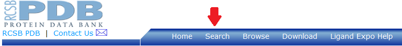
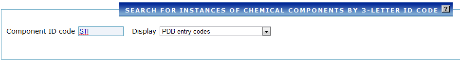
Ligand Expo (ligand-expo.rcsb.org), which was referenced in earlier versions of this lab, was retired on February 13, 2026. Its functionality has been integrated into the main RCSB PDB website. The screenshots below are from the original Ligand Expo interface and are preserved for historical reference — the current RCSB interface may look different.
The RCSB PDB (https://www.rcsb.org) provides chemical and structural information about small molecules within PDB entries. You can search for ligands directly on the main site.
Example 1: Find the ligand for c-Abl kinase (PDB ID: 1IEP)
- Go to https://www.rcsb.org and search for
1IEP. - On the structure summary page, scroll to the Small Molecules section.
- You will see that one of its ligands is imatinib (STI), an anti-cancer drug with 3-letter code
STI. - Click on
STIto view its ligand summary page, where you can find: - Molecular weight, formula, and formal charge
- 2D and 3D chemical structure diagrams
- Download links for SDF, PDB, and CIF coordinate files
- Links to external databases (PubChem, ChEMBL, DrugBank)
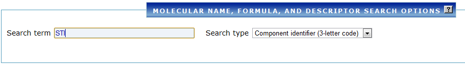
Example 2: Find PDB structures that contain STI (imatinib)
- On the RCSB PDB website, go to Advanced Search (https://www.rcsb.org/search/advanced).
- Under Chemical/Ligand, select Chemical ID and type
STI. - Run the search — you will see a list of all PDB structures that contain imatinib.
1.2 BindingDB
BindingDB (https://www.bindingdb.org) is a public database of measured binding affinities, focusing on interactions of drug-target proteins with small, drug-like molecules. As of 2026, it contains over 3.1 million binding measurements across 3,100+ target proteins.
Example 3: Find alternative drugs that may bind to Abl kinase
- Go to https://www.bindingdb.org
- Use the Quick Search → Choose target option, select
ABL, and click Go.
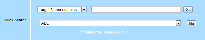
- The results page displays binding parameters like ΔG°, Ki, Kd, IC50, etc.
- Select a compound of interest (e.g., PD153035).
- You will see links to external databases (DrugBank, PubChem, Google Scholar, PDB).
- Following the DrugBank link provides: chemical formula, molecular weight, water solubility, mechanism of action, and downloadable SDF/PDB files.
1.3 ZINC Database
ZINC is a free database of commercially available compounds for virtual screening. The latest version, ZINC-22, contains billions of make-on-demand molecules.
- ZINC-22 (CartBlanche): https://cartblanche22.docking.org/
- ZINC-20 (smaller catalogs, in-stock): https://zinc20.docking.org/
Example 4: Find similar drugs to zoledronic acid (ZOL)
Another anti-cancer drug is zoledronic acid (ZOL), which targets farnesyl pyrophosphate synthetase.
- Find the structure of
ZOLfrom the RCSB PDB ligand page. - Go to https://cartblanche22.docking.org/
- Use the Similarity Search feature — paste the SMILES string of zoledronic acid.
- Set similarity to 80% and run the search.
- A list of structurally similar compounds is displayed, each with vendor availability and predicted properties.
Info
Other Useful Databases:
- PubChem (https://pubchem.ncbi.nlm.nih.gov) — NIH's open chemistry database with >100 million compounds, bioassay data, and direct SDF downloads.
- ChEMBL (https://www.ebi.ac.uk/chembl/) — Curated bioactivity database from the European Bioinformatics Institute.
- DrugBank (https://go.drugbank.com) — Comprehensive drug information including pharmacology, interactions, and targets.
2. Receptor Preparation in ChimeraX
Before docking, the receptor protein must be rigorously cleaned and prepared. ChimeraX provides the Dock Prep tool that automates most of this process. This section uses the skills from Lab 5–7 Milestones 3 & 4 — refer back to those sections for detailed explanations of selections, binding pockets, and structure editing.
Step 1: Fetch the Structure and Inspect It
Via Command Line:
# Fetch Abl kinase from the PDB
open 1iep

# Review metadata and chain inventory
log metadata
log chains
The Log panel will show that 1IEP contains:
- Chain A — Abl kinase protein
- STI (imatinib) — the co-crystallized ligand
- Water molecules (HOH) and possibly ions
Step 2: Identify the Ligand
# List all ligands in the structure
info residues ligand

# Select and inspect the imatinib ligand
select :STI
label sel residues
view sel
Step 3: Extract the Co-Crystallized Ligand (for Later Use)
Before cleaning the receptor, save the ligand coordinates — you will need them to define the binding box and to validate your docking results.
# Select only the STI ligand
select :STI

# Save it as a separate PDB file
save STI_from_crystal.pdb format pdb selectedOnly true
Tip
You can also download the ligand SDF file directly from the RCSB PDB ligand page for STI — this is often preferred because SDF files preserve bond orders and stereochemistry better than PDB format.
Step 4: Clean the Receptor
Remove everything that is not the protein receptor:
# Keep only chain A (if multiple chains exist)
delete ~#1/A

# Remove the co-crystallized ligand (we want to dock INTO the empty pocket)
delete :STI

# Remove solvent
delete solvent
Step 5: Run Dock Prep — The All-In-One Cleanup
Via GUI: Go to Tools → Structure Editing → Dock Prep. In the dialog:
- ✅ Delete solvent
- ✅ Delete non-complexed ions
- ✅ Delete alternate locations
- ✅ Standardize certain residue types
- ✅ Incomplete side chains → Replace using Dunbrack rotamer library
- ✅ Add hydrogens
- ✅ Add charges (select Gasteiger for Vina compatibility)
Click OK.
Via Command Line:
# Run the full Dock Prep pipeline with Gasteiger charges
dockprep #1 acMethod gasteiger
Info
What dockprep does in one command:
- Deletes water molecules and non-complexed ions
- Removes unused alternate locations (altlocs)
- Converts non-standard residues (e.g., selenomethionine → methionine)
- Repairs truncated sidechains using the Dunbrack rotamer library
- Adds explicit hydrogens with pH-aware protonation states
- Assigns Gasteiger partial charges and GAFF atom types (via Antechamber)
Warning
What Dock Prep does NOT do:
- Missing backbone segments — If entire loops are absent from the crystal structure, Dock Prep will not build them. Use Model Loops or AlphaFold for that.
- PDBQT conversion — ChimeraX cannot write PDBQT files. This requires external tools (covered in Section 4).
- Glycosylation removal — NAG, MAN, and other sugar residues must be deleted manually if unwanted (
delete :NAG,MAN,GAL).
Step 6: Save the Prepared Receptor
# Save as PDB (standard format)
save 1iep_receptor_cleaned.pdb format pdb

# Save as Mol2 (preserves the Gasteiger charges assigned by dockprep)
save 1iep_receptor_cleaned.mol2
Tip
The Mol2 format retains atomic partial charges in the file, whereas PDB format does not store charge information in the coordinate columns. For docking preparation pipelines that read charges from the input file, Mol2 is preferred.
3. Defining the Binding Box in ChimeraX
The docking search space is defined by a 3D rectangular grid box centered on the binding site. AutoDock Vina requires the box center (x, y, z) and size (x, y, z) in Ångströms.
Since we extracted the co-crystallized ligand position in Step 3, we can use it to define the box precisely.
Step 1: Reload the Ligand for Reference
# Open the saved crystal ligand alongside the cleaned receptor
open STI_from_crystal.pdb
Step 2: Create a Visual Bounding Box
# Select the reference ligand
select #2

# Create a simulated density map around the ligand (3 Å resolution, 5 Å padding)
molmap sel 3 edgePadding 5

# Draw a bright cyan outline box around the map
volume #3 showOutlineBox true outlineBoxRgb cyan

# Make the density invisible — we only want the box outline
transparency #3 100
Danger
Do not use the global ligand keyword here! If the structure has multiple ligands, the box will stretch to encompass all of them. Always target a specific ligand selection.
Step 3: Extract Grid Box Coordinates
# Get the bounding box min/max coordinates
info bounds sel
The Log panel will print the minimum and maximum corner coordinates. Calculate the Vina grid parameters:
- Center X = (x_max + x_min) / 2
- Center Y = (y_max + y_min) / 2
- Center Z = (z_max + z_min) / 2
- Size X = x_max − x_min + padding
- Size Y = y_max − y_min + padding
- Size Z = z_max − z_min + padding
Tip
Add 2–5 Å of padding to each dimension beyond the ligand bounding box. This ensures the search space is large enough to accommodate alternative binding orientations. A typical grid box for a drug-sized ligand is 20–30 Å per side.
Step 4: Record the Values
Write down (or copy from the Log) the center and size values — you will need them for the Vina configuration file in Section 6. For 1IEP/STI, typical values are approximately:
center_x = 15.0
center_y = 53.0
center_z = 16.0
size_x   = 20.0
size_y   = 20.0
size_z   = 20.0
(Your exact values will depend on the padding you choose.)
4. Setting Up the Docking Tools
4.0 Why a Python Environment is Required
ChimeraX excels at structure visualization, cleaning, and analysis — but it cannot produce PDBQT files, which are the input format required by AutoDock Vina. The PDBQT format extends PDB with two additional columns: partial charges (Q) and AutoDock atom types (T), plus a torsion tree that defines rotatable bonds in the ligand.
Historically, PDBQT conversion was performed using MGLTools / AutoDock Tools (ADT). However, MGLTools is no longer recommended for modern workflows because:
- It is written in Python 2, which reached end-of-life in January 2020
- It has not been actively maintained for several years
- It is extremely difficult to install on modern operating systems (especially macOS with Apple Silicon)
- It relies on deprecated libraries (old Tkinter, PMW, NumPy 1.x)
The modern replacement is Meeko, developed by the same Forli Lab at Scripps Research that maintains AutoDock Vina. Meeko is:
- Pure Python 3, installable via
pip - Uses RDKit for robust chemical perception (bond orders, stereochemistry, atom typing)
- Supports flexible residues, reactive docking, and modern PDBQT extensions
- Actively maintained alongside AutoDock Vina
4.1 Installing Python and Creating a Virtual Environment
macOS
Python 3 can be downloaded directly from the official Python website — no Homebrew or Xcode Command Line Tools required.
- Go to https://www.python.org/downloads/ and download the latest Python 3 installer for macOS.
- Run the
.pkginstaller. It will install Python 3 to/Library/Frameworks/Python.framework/and addpython3to your PATH. - Open Terminal (Applications → Utilities → Terminal) and verify:
python3 --version
- Create a working directory and virtual environment:
# Create a project directory
mkdir ~/docking_lab
cd ~/docking_lab

# Create a virtual environment
python3 -m venv vina-env

# Activate it
source vina-env/bin/activate

# Install Meeko and RDKit
pip install meeko rdkit

# Verify
mk_prepare_ligand.py --help
mk_prepare_receptor.py --help
Windows
- Go to https://www.python.org/downloads/ and download the latest Python 3 installer.
- Important: During installation, check "Add Python to PATH".
- Open PowerShell (search for "PowerShell" in the Start menu) and verify:
python --version
- Create a working directory and virtual environment:
# Create a project directory
mkdir $HOME\docking_lab
cd $HOME\docking_lab

# Create a virtual environment
python -m venv vina-env

# Activate it
.\vina-env\Scripts\Activate.ps1

# Install Meeko and RDKit
pip install meeko rdkit

# Verify
mk_prepare_ligand.py --help
mk_prepare_receptor.py --help
Tip
If PowerShell blocks script execution, run Set-ExecutionPolicy -Scope CurrentUser RemoteSigned first.
Linux (Ubuntu / Debian)
# Install Python 3 and venv (if not already present)
sudo apt update
sudo apt install python3 python3-venv python3-pip

# Create a project directory
mkdir ~/docking_lab
cd ~/docking_lab

# Create and activate virtual environment
python3 -m venv vina-env
source vina-env/bin/activate

# Install Meeko and RDKit
pip install meeko rdkit

# Verify
mk_prepare_ligand.py --help
mk_prepare_receptor.py --help
Warning
Always activate your virtual environment before running Meeko commands. If your terminal prompt does not show (vina-env), the commands will not be found. Re-activate with source ~/docking_lab/vina-env/bin/activate (macOS/Linux) or ~\docking_lab\vina-env\Scripts\Activate.ps1 (Windows).
4.2 Converting the Receptor to PDBQT (Meeko)
With your virtual environment activated and the cleaned receptor PDB from Section 2:
# Copy the cleaned receptor into your working directory (if not already there)
# Then convert to PDBQT:

mk_prepare_receptor.py --read_pdb 1iep_receptor_cleaned.pdb -o 1iep_receptor -p -a
Flags explained:
| Flag | Meaning |
|---|---|
--read_pdb |
Input PDB file |
-o |
Output base name (produces 1iep_receptor.pdbqt) |
-p |
Write PDBQT output |
-a |
Allow bad/non-standard residues (skip instead of crashing) |
The output file 1iep_receptor.pdbqt is your docking-ready receptor.
Info
Meeko's receptor preparation adds hydrogens automatically if they are missing, assigns Gasteiger charges, and determines AutoDock atom types. If you already added hydrogens and charges in ChimeraX (via dockprep), Meeko will use the existing protonation state.
4.3 Preparing the Ligand PDBQT (Meeko)
Option A: Download the Ligand SDF from RCSB
- Go to https://www.rcsb.org/ligand/STI
- Under Downloads, select Ideal SDF to get
STI_ideal.sdf. - Place it in your
~/docking_lab/directory.
Option B: Use the Ligand Extracted from ChimeraX
If you saved the crystal ligand in Section 2 as STI_from_crystal.pdb, you can use that — but SDF is preferred because it preserves bond orders.
Convert to PDBQT:
mk_prepare_ligand.py -i STI_ideal.sdf -o STI.pdbqt
Warning
Input requirements: The ligand must have explicit hydrogens and 3D coordinates. SDF files from RCSB typically meet both requirements. If you get errors about 2D coordinates, Meeko will attempt 3D embedding automatically — but always verify the geometry visually in ChimeraX afterward (open STI.pdbqt).
5. AutoDock Vina: Installation & Configuration
5.1 Installing AutoDock Vina
Download the pre-compiled binary for your operating system from the official GitHub releases page:
https://github.com/ccsb-scripps/AutoDock-Vina/releases
- Download the archive for your platform (e.g.,
vina_1.2.7_linux_x86_64,vina_1.2.7_mac_x86_64, orvina_1.2.7_win32). - Extract the archive — it contains the
vina(orvina.exe) executable. - Place the executable somewhere accessible. You can either:
- Copy it into your
~/docking_lab/directory, or - Add its location to your system PATH.
- Verify the installation:
# macOS / Linux (if vina is in the current directory)
./vina --version

# Windows (PowerShell)
.\vina.exe --version
5.2 The Configuration File
AutoDock Vina can accept all parameters as command-line flags, but using a configuration file (conf.txt) is cleaner and more reproducible. Create a file named conf.txt in your ~/docking_lab/ directory:
receptor = 1iep_receptor.pdbqt
ligand   = STI.pdbqt

center_x = 15.0
center_y = 53.0
center_z = 16.0
size_x   = 20.0
size_y   = 20.0
size_z   = 20.0

exhaustiveness = 8
num_modes = 9
energy_range = 3.0
(Replace the center and size values with the ones you calculated in Section 3.)
5.3 Key Parameters — Detailed
| Parameter | Default | Description |
|---|---|---|
exhaustiveness |
8 | Controls the thoroughness of the global search. Higher values (16, 32) explore more of the conformational landscape and are more likely to find the global minimum, but take proportionally longer. For production runs, use 32 or higher. For quick tests during learning, 8 is adequate. |
num_modes |
9 | Maximum number of binding poses (modes) to generate. The actual number returned may be fewer if distinct poses cannot be found within the energy range. |
energy_range |
3.0 | Maximum energy difference (kcal/mol) between the best and worst binding mode reported. Modes with scores worse than best_score + energy_range are discarded. |
5.4 Additional Parameters
| Parameter | Default | Description |
|---|---|---|
cpu |
0 (auto) | Number of CPU cores to use. 0 = use all available cores. |
seed |
0 (random) | Random seed for reproducibility. Set to a fixed integer (e.g., 42) to get identical results across runs. |
scoring |
vina |
Scoring function. Options: vina (default), vinardo, ad4 (AutoDock 4 scoring). |
spacing |
0.375 | Grid spacing in Ångströms. Smaller values increase resolution but slow down computation. |
min_rmsd |
1.0 | Minimum RMSD (Å) difference between reported poses. Poses closer than this are considered duplicates. |
max_evals |
0 (auto) | Maximum number of evaluations. 0 lets Vina decide based on exhaustiveness and molecule size. |
verbosity |
1 | Output verbosity. 0 = silent, 1 = normal, 2 = verbose. |
6. Running AutoDock Vina
Step 1: Verify Your Files
Ensure your ~/docking_lab/ directory contains:
docking_lab/
├── 1iep_receptor.pdbqt     # Prepared receptor (Section 4.2)
├── STI.pdbqt                # Prepared ligand (Section 4.3)
└── conf.txt                 # Configuration file (Section 5.2)
Step 2: Run the Docking
# Navigate to your docking directory
cd ~/docking_lab

# Run Vina (macOS / Linux)
./vina --config conf.txt --out STI_docked.pdbqt --log STI_log.txt

# Windows (PowerShell)
.\vina.exe --config conf.txt --out STI_docked.pdbqt --log STI_log.txt
Step 3: Understand the Output
Vina prints a results table like this:
mode |   affinity   | dist from best mode
     | (kcal/mol)   | rmsd l.b.| rmsd u.b.
-----+-------+-------+-------+-------
   1       -11.2      0.000      0.000
   2       -10.8      1.432      2.156
   3       -10.5      1.876      3.241
   ...
| Column | Meaning |
|---|---|
| mode | Pose number (1 = best predicted binding mode) |
| affinity | Predicted binding free energy in kcal/mol. More negative = stronger binding. |
| rmsd l.b. | Lower-bound RMSD from the best mode (symmetry-corrected) |
| rmsd u.b. | Upper-bound RMSD from the best mode |
Info
What is a good score? For drug-like molecules binding to protein targets, scores in the range of −7 to −12 kcal/mol are typical. The first mode (best affinity) is the most likely binding pose. However, docking scores are approximations — always validate with experimental data or molecular dynamics simulations.
The output file STI_docked.pdbqt contains all binding modes as separate MODEL entries.
7. Analyzing Docking Results in ChimeraX
ChimeraX has a built-in ViewDock tool that is specifically designed for interactive analysis of docking results, including AutoDock Vina PDBQT output.
Step 1: Open the Receptor and Docking Results
# Open the prepared receptor
open 1iep_receptor.pdbqt

# Open the docking results — ViewDock starts automatically
open STI_docked.pdbqt
When ChimeraX opens a multi-model PDBQT file, the ViewDock panel automatically appears. It lists each docked pose with its binding score.
Step 2: Browse Poses in ViewDock
- Click a row in the ViewDock table to display that pose and hide the others.
- Sort by column — click the score column header to rank poses.
- Rate poses — assign ratings (good / maybe / bad) using the buttons or hotkeys (
g,m,b). - Navigate — use the Up/Down arrow keys with the ViewDock panel focused to step through poses.
Step 3: Validate Against the Crystal Structure
If you saved the crystal ligand position (Section 2, Step 3), superimpose the best docked pose on it:
# Open the original crystal ligand
open STI_from_crystal.pdb

# Visualize both together
show #2.1   ; # Best docked pose (adjust model number as needed)
show #3     ; # Crystal ligand

# Color to distinguish
color #2.1 dodgerblue
color #3 gold

# Show as sticks for atomic detail
style #2.1,#3 stick

# Compute and display hydrogen bonds
hbonds #2.1 restrict #1 color green
Tip
RMSD Validation: The RMSD between the best docked pose and the crystal pose tells you how well the docking reproduced the experimental binding mode. An RMSD ≤ 2.0 Å is generally considered successful redocking (reproducing the known pose).
Step 4: Visualize the Binding Pocket Interactions
# Select the binding pocket (residues within 4 Å of the docked ligand)
select #2.1 :\< 4

# Show pocket residues as sticks, color by heteroatom
show sel
style sel stick
color sel byhetero

# Label key interacting residues
label sel residues

# Hydrogen bonds between ligand and receptor
hbonds #2.1 restrict #1 color cyan

# Contacts (van der Waals)
contacts #2.1 restrict #1 color orange

# Publication-quality rendering
lighting soft
graphics silhouettes true
view #2.1
Step 5: Save the Analysis
# Save a publication-quality image
save docking_result.png width 1920 height 1080

# Save the session for later work
save docking_session.cxs
8. Flexible Docking (Advanced)
In standard rigid-receptor docking, the protein atoms are frozen. Flexible docking allows selected receptor side chains to move during the search, better modeling induced-fit effects.
Concept
- You specify which receptor residues should be flexible (typically 3–6 residues lining the binding pocket).
- Meeko splits the receptor into two files:
receptor_rigid.pdbqt— the bulk of the protein (fixed)receptor_flex.pdbqt— the flexible side chains (movable)- Vina optimizes both the ligand and the flexible side chains simultaneously.
Step 1: Identify Flexible Residues
In ChimeraX, identify key residues in the binding pocket:
# Select residues within 4 Å of the ligand
open 1iep
select :STI :\< 4
label sel residues
Note the residue numbers and chain IDs (e.g., A:271, A:286, A:315, A:381).
Step 2: Generate Rigid + Flex PDBQT Files
# In your activated vina-env, with the cleaned receptor PDB:
mk_prepare_receptor.py --read_pdb 1iep_receptor_cleaned.pdb \
    -o 1iep_flex \
    -p \
    -a \
    -f A:271,A:286,A:315,A:381
This produces:
- 1iep_flex_rigid.pdbqt
- 1iep_flex_flex.pdbqt
Step 3: Run Flexible Docking
./vina --receptor 1iep_flex_rigid.pdbqt \
       --flex 1iep_flex_flex.pdbqt \
       --ligand STI.pdbqt \
       --config conf.txt \
       --out STI_flex_docked.pdbqt \
       --log STI_flex_log.txt
Warning
Flexible docking is significantly slower than rigid docking. Each additional flexible residue multiplies the search space. Limit flexible residues to only those directly involved in binding (3–6 residues maximum).
9. Python Showcase: Automated ChimeraX Docking Pipeline
You can script the entire ChimeraX preparation workflow in the Python shell (Tools → General → Shell):
from chimerax.core.commands import run

print("=== Automated Docking Preparation Pipeline ===")

# Step 1: Fetch and clean the receptor
_ = run(session, 'open 1iep')
_ = run(session, 'delete ~#1/A')       # Keep only chain A

# Step 2: Extract the ligand before removing it
_ = run(session, 'select :STI')
_ = run(session, 'save STI_from_crystal.pdb format pdb selectedOnly true')

# Step 3: Remove ligand and clean
_ = run(session, 'delete :STI')
_ = run(session, 'delete solvent')

# Step 4: Run Dock Prep (adds H, charges, fixes sidechains)
_ = run(session, 'dockprep #1 acMethod gasteiger')

# Step 5: Save the prepared receptor
_ = run(session, 'save 1iep_receptor_cleaned.pdb format pdb')
_ = run(session, 'save 1iep_receptor_cleaned.mol2')

# Step 6: Visualize the binding pocket for the box definition
_ = run(session, 'open STI_from_crystal.pdb')
_ = run(session, 'select #2')
_ = run(session, 'molmap sel 3 edgePadding 5')
_ = run(session, 'volume #3 showOutlineBox true outlineBoxRgb cyan')
_ = run(session, 'transparency #3 100')
_ = run(session, 'info bounds sel')

# Step 7: Render a publication image
_ = run(session, 'view #2')
_ = run(session, 'lighting soft')
_ = run(session, 'graphics silhouettes true')
_ = run(session, 'save docking_prep_overview.png width 1920 height 1080')

print("Preparation complete! Now run Meeko + Vina from the terminal.")
10. Summary of Key Commands
ChimeraX Commands
| Task | Command |
|---|---|
| Fetch a PDB structure | open 1iep |
| Inspect metadata | log metadata |
| List chains | log chains |
| List ligands | info residues ligand |
| Select a specific ligand | select :STI |
| Delete unwanted chains | delete ~#1/A |
| Delete solvent | delete solvent |
| Delete specific residues | delete :NAG,MAN |
| Run Dock Prep (Gasteiger) | dockprep #1 acMethod gasteiger |
| Add hydrogens only | addh |
| Add charges only | addcharge method gasteiger |
| Save as PDB | save file.pdb format pdb |
| Save as Mol2 (with charges) | save file.mol2 |
| Save selected atoms only | save file.pdb format pdb selectedOnly true |
| Create bounding box | molmap sel 3 edgePadding 5 |
| Show outline box | volume #N showOutlineBox true outlineBoxRgb cyan |
| Get bounding box coordinates | info bounds sel |
| Open docking results (ViewDock) | open results.pdbqt |
| Hydrogen bonds to receptor | hbonds #LIGAND restrict #RECEPTOR color green |
| Contacts to receptor | contacts #LIGAND restrict #RECEPTOR color orange |
Meeko CLI Commands
| Task | Command |
|---|---|
| Prepare receptor PDBQT | mk_prepare_receptor.py --read_pdb receptor.pdb -o receptor -p -a |
| Prepare receptor with flex | mk_prepare_receptor.py --read_pdb receptor.pdb -o receptor -p -a -f A:271,A:286 |
| Prepare ligand PDBQT | mk_prepare_ligand.py -i ligand.sdf -o ligand.pdbqt |
AutoDock Vina Commands
| Task | Command |
|---|---|
| Run docking (config file) | vina --config conf.txt --out output.pdbqt --log log.txt |
| Run flexible docking | vina --receptor rigid.pdbqt --flex flex.pdbqt --ligand lig.pdbqt --config conf.txt --out out.pdbqt |
11. SONLab Vina Prep Tool — All-in-One Docking Preparation
Important
Educational Note: The manual workflow above — preparing the receptor in ChimeraX, converting with Meeko, defining the binding box, running Vina from the command line — is designed to teach you what each step does and why it matters. In practice, you will use the SONLab Vina Prep Tool, which automates this entire pipeline in a single graphical application. Understanding the underlying steps is essential for troubleshooting, interpreting results, and adapting the workflow to non-standard scenarios.
The SONLab Vina Prep Tool is a comprehensive, cross-platform graphical desktop application developed at the Bioinformatics Branch of the SONLab Research Team, Middle East Technical University. It integrates every step of the docking preparation pipeline into a single interface.
Features
| Feature | Description |
|---|---|
| Receptor Preparation | 12-step automated pipeline: PDB download, chain selection, altloc removal, residue standardization, missing atom repair, missing loop reconstruction, water/ion/glycosylation removal, hydrogen addition, charge assignment, and PDBQT conversion — all in one click. |
| 3D Binding Box Viewer | Interactive 3Dmol.js-based molecular viewer for visually defining the docking grid box by selecting ligand centroids or clicking atoms. |
| Ligand Preparation | Converts SMILES, SDF, or Mol2 files into docking-ready PDBQT format with automatic 2D→3D conversion, hydrogen addition, and charge assignment. |
| Flexible Docking | Select flexible side chains manually or auto-detect residues inside the binding box. Automatically generates rigid + flex PDBQT file pairs. |
| Execution Manager | Configure exhaustiveness, energy range, scoring functions, and multiple seeds. Launch AutoDock Vina directly from the UI. Results are organized by ligand, exhaustiveness, and seed with automatic CSV summary generation. |
| Cross-Platform | Runs on macOS (.dmg), Windows (Setup.exe), and Linux (.AppImage). |
Installation
Pre-built application binaries will be provided to you by your instructor for your operating system:
| Platform | Format | Installation |
|---|---|---|
| macOS | .dmg |
Open DMG → drag to Applications |
| Windows | Setup.exe |
Run installer wizard |
| Linux | .AppImage |
chmod +x *.AppImage → run directly |
Note
The SONLab Vina Prep Tool does not bundle AutoDock Vina itself. You must download Vina separately (Section 5.1) and point the Execution tab to the vina executable.
Quick Walkthrough with 1IEP
- Receptor Tab — Enter PDB ID
1IEP, select chain A, click Prepare. The tool downloads the structure, cleans it through 12 automated steps, and produces the receptor PDBQT. - Box Viewer — Click Open Viewer. The 3D viewer shows the receptor with the co-crystallized ligand. Click on the ligand to auto-center the binding box. Adjust box dimensions if needed.
- Ligand Tab — Load
STI_ideal.sdf, click Convert. The ligand PDBQT is generated. - Execution Tab — Set exhaustiveness to 32, select the receptor/ligand/box files, and click Run Docking.
- Results — Open the output PDBQT in ChimeraX for visualization and analysis (Section 7).
12. References
- Trott O, Olson AJ. AutoDock Vina: Improving the speed and accuracy of docking with a new scoring function, efficient optimization, and multithreading. J Comput Chem. 2010;31(2):455-461.
- Eberhardt J, Santos-Martins D, Tillack AF, Forli S. AutoDock Vina 1.2.0: New Docking Methods, Expanded Force Field, and Python Bindings. J Chem Inf Model. 2021;61(8):3891-3898.
- Wang J, Wang W, Kollman PA, Case DA. Automatic atom type and bond type perception in molecular mechanical calculations. J Mol Graph Model. 2006;25(2):247-260.
- Wang J, Wolf RM, Caldwell JW, Kollman PA, Case DA. Development and testing of a general amber force field. J Comput Chem. 2004;25(9):1157-1174.
- AutoDock Vina Documentation — Official Read the Docs.
- Meeko — Molecular Docking Preparation — Forli Lab, Scripps Research.
- ChimeraX Dock Prep Documentation — UCSF RBVI.
- RCSB PDB — Research Collaboratory for Structural Bioinformatics.
- BindingDB — Binding Database.
- ZINC-22 — Free database for virtual screening.