Week 5-7 - UCSF ChimeraX

Welcome to the enhanced ChimeraX tutorial. ChimeraX is the next-generation successor to UCSF Chimera, offering drastically improved graphics, ability to handle massive structures intuitively, integrated AlphaFold predictions, and a comprehensive Python 3 API.

---

Milestone 1: Introduction, Fetching Structures, and Basic View Manipulation

1.1 Getting Started

When you open ChimeraX, you will see a main 3D graphics window, a Command Line at the bottom, and typically a toolbar at the top. The graphical user interface (GUI) and the command line work seamlessly together. Whatever you can do in the GUI, you can do with a command, and vice-versa.

Tip

Educational Tip: Why use the command line? While clicking around is great for exploration, commands allow you to reproduce your exact workspace, automate repetitive tasks, and easily write scripts for computational pipelines.

1.2 Fetching an Experimental Structure (PDB)

Let's fetch Quinine Reductase II (PDB ID: 2QX4), an enzyme that binds specific drugs.

Via GUI:

1. Go to File → Fetch by ID...
2. In the resulting dialog, ensure PDB is selected.
3. Type 2QX4 and hit Fetch.

Via Command Line: In the command line at the bottom, simply type:

open 2qx4

Info

What is a PDB file? The Protein Data Bank (PDB) provides text files containing 3D coordinates (X, Y, and Z) of every atom, derived from physical experiments.

Substructures: A single PDB file isn't just a protein! It can contain multiple Chains (individual protein/RNA molecules), Ligands (small molecules/drugs like FAD or Quinine), and Solvent (water molecules). You can view and manage these components dynamically by opening the Model Panel via Tools → General → Model Panel.

1.3 Evaluating Metadata and Chains

Before attempting to manipulate a complex structure, it is incredibly helpful to evaluate exactly what you just downloaded.

1. Extracting Literature and File Metadata (Note: There is no direct GUI button that builds this specific text table; CLI extraction is the ChimeraX standard for deep metadata). To view exactly where this structure came from, its exact PDB title, experimental method, and primary citation:

log metadata

2. Reviewing the Chain Inventory To get a highly readable, interactive table of every sequence/polymer chain present (including length, chain ID, and descriptions) directly in your Log:

log chains

Tip

The table output by log chains contains interactive hyperlinks! Clicking the links directly in the Log panel will automatically select and focus on that sequence in the 3D window.

1.4 Basic View Manipulation (Mouse Controls)

Once the structure is loaded, you can manipulate the view:

• Rotate: Left-click and drag on the structure.
• Translate (Pan): Middle-click (or right-click) and drag to move the protein across the screen.
• Zoom: Use the scroll wheel to zoom in and out. Alternatively, on a trackpad, use a two-finger pinch.

You can reset the view at any time using the command line:

view

1.5 Using the Side View for Clipping and Sectioning

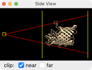
Sometimes, to peer deep inside a protein's interior (like examining a buried binding pocket), you need to physically "slice" through the structure. ChimeraX provides the Side View tool for this.

Via GUI: Go to Tools → General → Side View (or click the Side View icon on the Graphics toolbar). A miniature side-on schematic of your scene will appear showing: - A square on the left representing your eye position (drag it to zoom). - Two vertical lines representing the near and far clipping planes.

Drag the near clipping plane line to the right to slice into the front of the structure, progressively revealing buried interior features. Drag the far plane left to trim the back. Tick the clip checkboxes to activate/deactivate each plane.

Via Command Line:

# Activate the near clipping plane and slice 10 Å into the structure
clip near 10

# Turn off all clipping to restore the full view
~clip

1.6 Fetching Predicted Structures (AlphaFold)

ChimeraX directly integrates with the AlphaFold database, allowing you to instantly load AI-predicted structures without needing experimental data!

Let's try fetching the AlphaFold prediction for a human protein, like Human TP53 (Cellular tumor antigen p53). In the command line, type:

alphafold match P04637

(P04637 is the UniProt ID for this protein).

Warning

Educational Tip: Experimental structures (from the PDB) are ground truth snapshots of proteins. AlphaFold models are predictions. ChimeraX colors AlphaFold structures by a confidence score (pLDDT) where blue is highly confident, and red/orange is unstructured/low confidence. Always pay attention to these colors!

Now let's explicitly add a Color Key Legend so we know exactly what these colors mean!

Via GUI:

1. Go to Tools → Depiction → Color Key.
2. A dialog will open where you can adjust the gradient. For AlphaFold, you match it to the red-to-blue confidence scale. Start by setting "Number of colors/labels" to 5.
3. Then adjust the colors from bottom to top as: Red, Orange, Yellow, Cornflower Blue, Blue.

Via Command Line: This is often much faster and more precise. You can build a manual key by typing:

key red:low orange: yellow: cornflowerblue: blue:high

Or you can use the super-convenient built-in AlphaFold preset!

key alphafold

(You will now see a legend appear in the graphics window, serving as a guide for your AlphaFold model's confidence scores).

Adding a Title to Your Legend: The key command generates the color bar, but it does not have a built-in title parameter. To add a descriptive title label above the key, use the 2dlabels command to float a standalone text object on the screen.

Via GUI: Go to Tools → Depiction → 2D Labels and Arrows. Type your title text in the dialog, set the font size, and click to place it on screen. You can then use the Use mouse... checkbox or the Right Mouse → Move Label mode to drag it precisely above the color bar.

Via Command Line:

# Place a title above the default key position
2dlabels text "Confidence (pLDDT)" xpos 0.7 ypos 0.14 size 24 bold true

1.7 Managing the Working Directory

When you save files or open local structures with relative paths, ChimeraX uses a working directory as the root location. By default, this is ~/Desktop on Mac/Windows and ~/ on Linux. Understanding and changing it is critical for organized project work.

Via GUI: Go to File → Set Working Folder.... A file browser will open, allowing you to navigate to your desired project folder.

Via Command Line:

# Check the current working directory
pwd

# Change to a specific project folder
cd /Users/yourname/Documents/MyProject

# Change back to your home directory
cd

# Use a file browser to pick interactively
cd browse

Tip

Why does this matter? When you type save my_protein.pdb, the file is created inside the working directory. If you don't set it first, your files could end up scattered on your Desktop! Always set your working directory at the start of a session. You can also drag-and-drop a folder icon onto the command line to paste its path automatically.

1.8 Python Showcase: Basic Execution

ChimeraX isn't just a C++ GUI program; it is deeply integrated with Python 3. Everything ChimeraX does can be invoked via Python.

To open the Python shell interface:

1. Go to Tools → General → Shell

You will see an IPython prompt (e.g., In [1]:). You can run any ChimeraX command directly through the run function by passing the active session. This is useful for writing simple dynamic scripts or loops.

In the Shell, type:

# Import the run function to avoid IPython magic command conflicts
from chimerax.core.commands import run

# First, let's close all open models to clean our workspace.
# We assign the result to a variable (_) to safely bypass IPython's internal "run" command.
_ = run(session, 'close session')

# Now let's fetch 2QX4 using Python!
_ = run(session, 'open 2qx4')

1.9 Tracking and Reverting Changes

Unlike some other software that uses a visual "state tree" (like PyMOL or Maestro) to save distinct snapshots as you work, ChimeraX tracks states and models centrally but relies on standard commands to revert mistakes:

• Undo: If you make a mistake (like changing a color), you can easily revert it using the undo command or hitting Ctrl+Z (Cmd+Z on Mac).
• History: To see a log of the commands you've executed, open Tools → General → File History or Tools → General → Log. The Log is your primary timeline of actions, errors, and calculated results.

This concludes Milestone 1! Let's continue to the next part.

---

Milestone 2: Visualization Styles, Lighting, and Coloring

2.1 Exploring Representation Styles

Proteins are too complex to display every atom as a ball simultaneously (unless you really want to!). Instead, we use different representation styles to highlight different features.

With 2QX4 loaded, let's explore styles:

Via GUI: Go to the Molecule Display tab in the top Toolbar. Here you can click icons to Show/Hide Cartoons , Atoms , and Surfaces .

Via Command Line:

• Show as a cartoon (ribbon): cartoon (and hide atoms: hide atoms)
• Show all atoms as sticks: show atoms ; style stick
• Show all atoms as spheres: style sphere
• Show the molecular surface: surface

Showing and Hiding Surfaces for Specific Atoms/Residues: You don't have to surface the entire protein! ChimeraX allows you to create or show/hide surface patches for targeted selections.

Via GUI: First select the atoms of interest (e.g., Select → Structure → Ligand), then go to Actions → Surface → Show (or Hide).

Via Command Line:

# Show a surface only around the ligand
surface ligand

# Show the surface patch for specific residues within an existing chain surface
surface :10-50

# Hide the surface patch for a specific range
surface hide /A:5-38

# Remove a surface entirely
surface close

Tip

Educational Tip: When should you use what? - Cartoons are best for seeing the overall 3D fold and secondary structures (alpha-helices and beta-sheets). - Sticks/Spheres are necessary when you want to look closely at how specific side-chains interact in a binding pocket. - Surfaces are perfect for visualizing the overall shape and identifying cavities or tunnels where drugs might bind.

2.2 Coloring Your Molecule

ChimeraX provides a sophisticated coloring system that gives you precise control over your protein's appearance.

Info

Educational Tip: What do the preset default coloring schemes in the GUI represent? - By Heteroatom (Element): Standard organic chemistry colors (Oxygen=red, Nitrogen=blue, Sulfur=yellow). Essential for examining specific chemical interactions like hydrogen bonds! - Rainbow: Colors the protein chain sequentially from the N-terminus (blue) to the C-terminus (red). This helps trace the continuous macroscopic fold of a polypeptide chain. - Electrostatic (coulombic): Maps the surface charge (Red = Negative, Blue = Positive, White = Neutral). Highly useful for predicting where oppositely-charged ligands or nucleic acids might bind. - Hydrophobicity (mlp): Maps the Molecular Lipophilicity Potential (Golden/Orange = Hydrophobic, Cyan/Blue = Hydrophilic). Perfect for pinpointing greasy membrane-insertion regions or hydrophobic drug-binding pockets. - B-factor (color bfactor): Colors by thermal mobility/flexibility, using data directly from the PDB file. (Blue = highly rigid/ordered regions, Red = highly flexible/disordered loops). - By Chain: Assigns a different generic color to every separate chain to easily tell interacting subunits apart.

Via GUI: Select the Molecule Display tab. You'll find icons for all of the above options:

Icon	Coloring Scheme
	Rainbow (N→C)
	Electrostatic (Coulombic)
	Hydrophobicity (MLP)
	B-factor (flexibility)
	Color by Chain
	Color by Heteroatom

Via Command Line:

• Color the secondary structure elements individually (helices pink, sheets yellow, loops white):

  color helix pink
  color strand yellow
  color coil white
  

• Color the two different protein chains with distinct colors:

  color bychain
  

• Color atoms by their heteroatom type:

  color byhetero
  

• Trace the chain direction from N-terminus to C-terminus:

  rainbow
  

• Color the surface by electrostatic charge (ensure your surface is visible first!), and generate its legend:

  surface
  coulombic
  key redblue
  

• Color the surface by Hydrophobicity (Lipophilicity) and generate its legend:

  mlp
  key lipophilicity
  

• Color atoms by their thermal flexibility (B-factor):

  color bfactor
  

2.3 Targeted Coloring and Displaying Bonds

Sometimes you want to analyze very specific structural interactions rather than looking at the global picture. You can specifically target your color and display commands to residues, atoms, and bonds.

1. Targeting Specific Residues and Atoms: ChimeraX uses a powerful selection syntax where : means residue and @ means atom name.

• Color all Lysine residues cyan:

  color :LYS cyan
  

• Color residues 10 through 50 bright green:

  color :10-50 green
  

• Color only the alpha-carbons (CA) of the entire protein magenta:

  color @CA magenta
  

2. Showing and Coloring Primary Covalent Bonds: When you color an atom, its attached bonds typically take on half of that color (called "halfbond" mode). You can show and color bonds specifically:

• Show all atoms and bonds for specifically Lysine residues as sticks:

  show :LYS  
  style :LYS stick
  

• Force all covalent bonds to be colored grey globally, regardless of their parent atom's color, by using the target b (bonds) option:

  color grey target b
  

3. Detecting and Coloring Hydrogen Bonds: ChimeraX automatically establishes geometric criteria to find secondary hydrogen bonds, rendering them as dashed lines.

• Find all hydrogen bonds in the structure and color the dashed lines yellow:

  hbonds color yellow
  

• Find only the hydrogen bonds that the protein makes with a ligand, and color them red:

  hbonds protein restrict ligand color red
  

• To remove the hydrogen bonds from the screen:

  ~hbonds
  

4. Selecting Atoms Participating in H-Bonds: After calculating hydrogen bonds, you may want to actually select the donor/acceptor atoms (e.g., to color them, label them, or measure distances). Append the select true flag:

hbonds select true

This will highlight the specific atoms making H-bonds and deselect everything else. To expand that selection from individual atoms up to their full parent residues, use the Up Arrow key on your keyboard, or equivalently:

select up

Tip

The "Select Up" Logic: In ChimeraX, selections follow a hierarchy: Atom → Residue → Chain → Model. Pressing the Up Arrow key after any selection always broadens it one level up (from atoms to residues, from residues to chains, etc.). Conversely, Down Arrow narrows it back down.

2.4 Advanced Lighting and Graphics (ChimeraX Feature)

One of the biggest reasons to switch from Chimera to ChimeraX is the rendering engine. ChimeraX uses advanced lighting techniques like ambient occlusion (soft shadows) and silhouettes (black outlines that drastically improve depth perception).

Let's make our protein look stunning! (GUI: click and in the Lighting toolbar tab)

graphics silhouettes true
lighting soft

(Notice how the deeper crevices of the protein are now cast in soft, realistic geometric shadows!).

Via GUI: You can toggle presets via the Lighting tab in the top Toolbar by clicking "Soft" or "Flat", and turn on "Silhouettes".

2.5 Python Showcase: Programmatic Coloring

Let's use the Python shell (Tools -> General -> Shell) to see how scripts can automate this logic.

from chimerax.core.commands import run

# Change the background color using the command function
_ = run(session, 'set bgColor white')

# Enable gorgeous lighting via script
_ = run(session, 'graphics silhouettes true')
_ = run(session, 'lighting soft')

# Let's dynamically color chain A cyan and chain B orange
_ = run(session, 'color /A cyan')
_ = run(session, 'color /B orange')

This concludes Milestone 2! Let's narrow our focus to the ligand and its immediate surroundings.

---

Milestone 3: Selections, Binding Pockets, and Interaction Labels

3.1 Selecting the Ligand and Identifying its Binding Pocket Zone

To see how a potential drug interacts with the protein, we first need to identify the binding pocket. But before we can click or select a ligand, we need to know exactly what ligands exist in the structure!

Step 1: Finding the Components

Via GUI: Simply click Select → Structure in the top menu and observe the categorical sub-menus. If Ligand, Solvent, or Ions is actively populated with options, you know those elements exist in the file!

Via Command Line: For a precise, readable text readout (including chain naming), we can ask ChimeraX to print a master inventory:

• List all ligands: info residues ligand
• List all solvent molecules (waters/buffers): info residues solvent
• List all metal ions: info residues ions

(Looking at the output in the log will give you their distinct residue names and chain numbering!)

Step 2: Selecting the Targets

Via GUI:

1. Select the ligand: Go to Select → Structure → Ligand.
2. Select the pocket (zone): Go to Select → Zone. Check the box for "Select all residues with any atom within [ 5.0 ] Å of currently selected atoms", and hit OK.

Via Command Line:

• Select just the ligand:

  select ligand
  

• Select the binding pocket (any residue within 5 Å of the ligand):

  select ligand :< 5
  

3.2 Isolating the Pocket and Applying Colors (Back Connection)

Now that the pocket is selected (the command line refers to the active selection as sel), let's use the skills we learned in Milestone 2 to focus precisely on these interactions and visualize them properly!

Via GUI:

1. Isolate: To hide everything except what we've selected, use the menus: Select → Invert (all models), then Actions → Atoms/Bonds → hide. Re-invert the selection so our binding pocket is selected again.
2. Display style: Go to the Molecule Display toolbar and click the Sticks icon to show all the side-chains in our pocket.
3. Color: While still in the Molecule Display toolbar, select the "Color Heteroatoms" icon to color-code the atoms (Oxygen=red, Nitrogen=blue) for assessing H-bonds.

Via Command Line: We can do all of that much faster with the following sequence:

hide ~sel
show sel
style sel stick
color sel byhetero

(Notice how using ~sel lets us quickly hide the unselected regions, and color sel byhetero applies the Milestone 2 organic chemistry coloring directly to our binding pocket!).

3.3 The "High Contrast" Context View (Space-filling & Metals/Glycosylations)

Sometimes zooming in too much loses the structural context of the whole molecule. Let's create a high-contrast view where the whole protein is visible as a faint cartoon, but our targets (ligands, metal ions, or glycosylations) pop out in full 3D space!

Via GUI:

1. Protein Context: Show the overall structure as a cartoon, color it white, and make it partially transparent via Molecule Display tools and Actions → Color → Transparency.
2. Space-filling Targets: Find your ligand, metal ions, or glycans via Select → Structure, then click the Sphere (space-filling) icon.
3. Interactions: Go to Tools → Structure Analysis → H-Bonds (and Contacts), using the dialog checkboxes to restrict calculations only to the currently selected items.

Via Command Line: Let's show the whole protein cartoon in white, but draw the ligand, any metal ions (ions), and standard glycosylations (like NAG or MAN sugars) as massive, high-contrast spheres!

# Make the background protein ghost-like
show protein ribbons
color protein white
transparency protein 50

# Highlight ligands, metal ions, and typical glycosylation sugars
select ligand | ions | :NAG,MAN
style sel sphere
color sel magenta

(Notice how the | operator acts as "OR", grabbing all of these distinct structural elements at once!)

Now let's compute all interactions—connecting our high-contrast targets to the ghost protein.

# Hydrogen bonds (Dashed cyan lines)
hbonds sel restrict protein color cyan

# Broad structural contacts / metal coordination (Dashed orange lines)
contacts sel restrict protein color dark orange

Interchain Interactions (Protein-Protein Interface Analysis): When studying multi-chain complexes (like dimers, antibody-antigen pairs), you often need to visualize only the bonds crossing between two chains, ignoring internal contacts:

# Hydrogen bonds crossing between Chain A and Chain B
hbonds /A restrict /B reveal true color green

# Salt bridges only crossing between chains (charged residue pairs)
hbonds /A restrict /B saltOnly true color magenta

# All steric contacts (van der Waals touches) at the interface
contacts /A restrict /B color dark orange

Displaying Disulfide Bonds: Cysteine residues can form covalent S-S (disulfide) bridges that physically staple protein chains (or loops within the same chain) together. ChimeraX recognizes these automatically from the coordinate file. To highlight them:

Via GUI: Go to Select → Chemistry → Functional Group → Disulfide. Then use Actions → Atoms/Bonds → Show and style them as sticks.

Via Command Line:

# Select all atoms participating in disulfide bonds
select disulfide

# Show them as prominent sticks and color the sulfur atoms yellow
show sel
style sel stick
color sel yellow target a

Info

The functional-group keyword disulfide selects only the cysteine residues that are actually participating in a covalent S-S bridge. Free (reduced) cysteines are excluded! You can verify this distinction yourself with the atomspec select :cys@sg & ~disulfide to find only the non-bridging cysteine sulfurs.

3.4 Adding 3D Interaction Labels

To identify which residues are making up the pocket so we can study them, we can label them.

Via GUI: Go to Right Mouse → Label , then click on any residues you want to identify. Alternatively, with your pocket still selected, go to Actions → Label → Residues.

Via Command Line:

• Label the currently selected residues (our binding pocket):

  label sel residues
  

• To clear the labels to clean up the view:

  ~label
  

3.5 Python Showcase: Automating Pocket Isolation

Combining selection, display changes, and coloring via the shell:

from chimerax.core.commands import run

# 1. Automatically grab the binding pocket
_ = run(session, 'select ligand :< 5')

# 2. Hide everything else and show the pocket as sticks
_ = run(session, 'hide ~sel')
_ = run(session, 'show sel')
_ = run(session, 'style sel stick')

# 3. Label the residues and color by heteroatom!
_ = run(session, 'label sel residues')
_ = run(session, 'color sel byhetero')

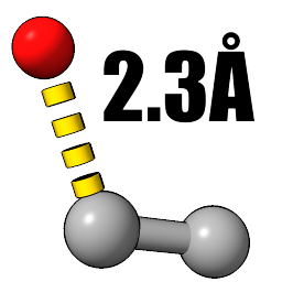
3.5 Measuring Distances and Angles

Via GUI: To explicitly track a distance or angle with a geometric dashed line and a measurement label in your 3D view:

1. Distance: Go to the Right Mouse toolbar → Measure Distance . Because you assigned this tool to the right mouse button, you must right-click on two atoms in the graphics window. A distance monitor will appear!
2. Angle: Go to the Right Mouse toolbar → Measure Angle. Right-click three atoms in sequence.

Via Command Line: (Note: You need to specify exact atoms. You can find atom names by pausing your mouse over them in the 3D viewer).

• Measure the distance between Atom A and Atom B:

  distance /A:15@O /A:18@N
  

• Measure the angle between three atoms:

  angle /A:15@C /A:15@O /A:18@N
  

Info

Why can't I see my angle? Unlike distances, which ChimeraX physically draws on the structure as visual dashed cylinders, geometric angles do not generate graphical 3D arcs. The angle command computes the scalar value and exports it strictly to your Log panel as text. - Choosing 3 atoms calculates the standard Valence Angle. - Choosing 4 atoms (using the torsion command or selecting 4 atoms in the GUI) calculates the Torsion (Dihedral) Angle.

How to Remove Measurements:

Via GUI: Go to Tools → Structure Analysis → Distances (or Angles/Torsions). This opens a structural measurement tab where you can select specific measurements in the table and click the Delete button.

Via Command Line:

• To instantly wipe all active measurement monitors from the workspace:

  ~distance
  ~angle
  

3.6 Ligand Size & Docking Bounding Boxes

When designing a drug, knowing the volume of the pocket—and defining a standard 3D search space (a docking grid box)—is crucial for tools like AutoDock Vina.

Part 1: Measuring Ligand Volume Because mathematical surfaces are mapped as broad geometric layers over an entire structural model, bounding volume tools require us to pass the model identifier (like #1) instead of an atomic name.

Via GUI: First, generate your surface using the tools we learned. Then, go to Tools → Volume Data → Measure Volume and Area. Select your newly generated surface from the dialog window to calculate its volume.

Via Command Line:

# Generate a surface exclusively around your targeted selection
surface sel

# Measure the physical spatial volume enclosed by that surface (in ų)
measure volume #1

Part 2: Drawing a Docking Grid Bounding Box To visually define a 3D rectangular search space for molecular docking (like establishing a grid box for AutoDock Vina), we can wrap our ligand in a simulated map and extract the exact geometrical bounding box coordinates. (Note: Creating isolated algorithmic bounding boxes and density maps is inherently computational and is exclusively driven via the command line interface).

Danger

Do not use the global ligand keyword here! If a protein has multiple ligands scattered across its surface, the box will stretch massively to encompass all of them. Always target a single ligand first, then run the bound command on that selection (sel).

How to isolate a specific ligand: - Via GUI: Hold Ctrl (or Cmd on Mac) and Left-Click on any atom of your target ligand. Then, press the Up Arrow on your keyboard to instantly expand the selection to the entire ligand molecule! - Via CLI: Pass the specific residue name or unique residue ID directly to the selection command (e.g., select :ATP or select /A:205).

(Note: This map-generation process creates a new model, usually designated as model #2. Adjust #2 if you have multiple structures open).

# 1. Create a simulated density map constrained tightly around your selected ligand
molmap sel 3

# 2. Draw a bright cyan outline box precisely around the limits of that map
volume #2 showOutlineBox true outlineBoxRgb cyan

# 3. Make the internal density map totally transparent, leaving only the docking box!
transparency #2 100

Tip

Adjusting the Grid Dimensions:
If the generated boundary is too tight or too wide, you can interactively resize it! Go to the Right Mouse toolbar → Crop Volume . Then simply right-click and drag any face of the cyan outline box to dynamically expand or shrink your docking search space. Alternatively, you can add edgePadding <value> to your molmap command to mathematically add a universally thick buffer region to the bounds.

Part 3: Extracting Grid Box Center and Size for External Tools Docking programs like AutoDock Vina, Glide, or GOLD require you to input the exact grid box center (x, y, z) and size (x, y, z) in Angstroms. ChimeraX can calculate these values directly!

The Mathematical Match for Docking Grids: There is a strict mathematical distinction when finding the "center" of a ligand. * Center of Mass (measure center sel): The mass-weighted center (heavier atoms pull the center point toward them). * Centroid (define centroid sel): The non-mass-weighted geometric center (raw average of all X, Y, Z coordinates). * Bounding Box Midpoint: The exact mathematical center of the 3D grid extents.

Because docking programs like AutoDock Vina mathematically build a symmetrical grid box by extending outward from a center coordinate by a given size, providing the Center of Mass or Centroid will result in a shifted, offset box that does not match the visual cyan grid box you drew with molmap.

To perfectly recreate your visual grid in Vina, both the Size and Center must be derived exclusively from the bounding box limits.

Via Command Line:

# Get the bounding box dimensions (xyz min and max corner coordinates)
info bounds sel

The info bounds command prints the minimum and maximum corner coordinates of the rectangular bounding box directly to the Log.

Tip

Perfecting the Vina Config File:
To ensure your Vina grid box perfectly overlays your ChimeraX visual box, use the info bounds sel output for all math: - Size X → x_max - x_min - Center X → (x_max + x_min) / 2 (Repeat these calculations for the Y and Z axes)

Part 4: Saving Selections for Future Reuse After carefully building a complex selection (like a binding pocket), you don't want to lose it! ChimeraX allows you to name a selection so you can recall it instantly in future commands, and also export the selected atoms to a file.

Naming Selections (In-Session Recall):

Via GUI: Go to Select → Define Selector. Name the current selection and it will appear under Select → User-Defined Selectors for easy recall.

Via Command Line:

# Name the current selection as "pocket" (frozen = locked to current atoms)
name frozen pocket sel

# Now use "pocket" anywhere you'd normally write a spec!
color pocket magenta
hbonds pocket restrict protein

# List all saved names
name list

Exporting Selected Atoms/Residues to a File: You can write only the selected atoms to a PDB file using the selectedOnly flag:

save binding_pocket.pdb format pdb selectedOnly true

Reporting Selection Details to a Text File: To save a detailed inventory of the selected items (residue names, numbers, chains) for documentation:

# Report selected atoms to the Log
info selection

# Report selected residues
info selection level residue

# Save to a file directly
info selection level residue saveFile pocket_residues.txt

3.7 The "Classic" Ligand Interaction Snippet

Let's pull together everything we've learned into one master "snippet". This is the classic workflow you will see in professional software like Maestro or PyMOL to generate a perfect, publication-ready view of a ligand embedded in its receptor.

Try running this sequence line-by-line:

# 1. Clean the slate
hide all
~surface
~hbonds

# 2. Highlight the ligand as Ball-and-Stick
show ligand
style ligand ball

# 3. Show interacting residues (within 4 Å) as sticks
show ligand :< 4
style sel stick

# 4. Color by heteroatom for chemical clarity
color sel byhetero

# 5. Draw hydrogen bonds just between the ligand and protein
hbonds ligand restrict protein color green

# 6. Smooth the lighting and zoom the camera perfectly to the ligand
lighting soft
graphics silhouettes true
view ligand

(You now have a flawless, high-contrast structural interaction graphic!)

3.8 Python Showcase: Programmatic Measurements

from chimerax.core.commands import run

# Calculate the volume programmatically on our selected ligand
_ = run(session, 'surface sel')

# We can capture the output of this run command to parse the volume value 
# or bounding box coordinates to feed directly into a Python docking pipeline!
_ = run(session, 'measure volume #1')

---

This concludes the massive Milestone 3. You are now a master of spatial selections, interaction networking, and bounding geometry.

---

Milestone 4: Structure Editing and Data Cleanup

Before any computational experiment (like docking or molecular dynamics), experimental structures must be rigorously "cleaned." Crystallography often captures crystallization buffers, split atomic positions, and artifacts that will immediately crash computational pipelines.

4.1 Stripping Solvents and Artifacts

Docking grids and simulation boxes require your protein to be a pristine receptor. We must remove floating waters, buffer salts, duplicate chains, and often the co-crystallized ligand itself (so we can dock new drugs into the empty pocket!).

Via GUI: Go to Select → Structure → Solvent (or Ions / Ligand). Once selected, go to Actions → Atoms/Bonds → delete.

Via Command Line:

• Remove all water/buffer molecules:

  delete solvent
  

• Remove all ligands (to empty out the binding pocket for a docking run):

  delete ligand
  

• Delete an unwanted, duplicated chain B (if your biological unit only requires chain A):

  delete /B
  

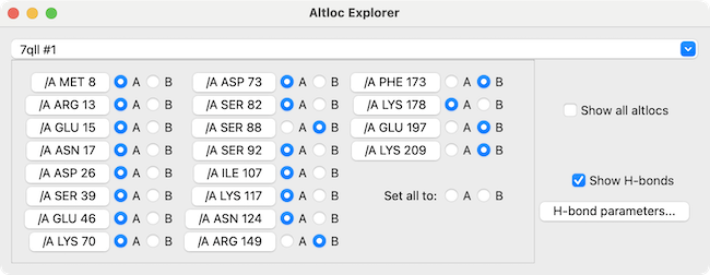
4.2 Resolving Alternate Locations (AltLocs)

High-resolution X-ray structures occasionally freeze flexible sidechains in multiple overlapping conformations (e.g., a Tyrosine toggling between two rotamer positions). Computational software crashes if an atom exists in two places at once. We must understand and resolve them.

Step 1: Finding Which Residues Have Alternate Locations

Via GUI: Go to Tools → Structure Analysis → Altloc Explorer. This dialog lists every residue with alternate conformations and shows which one is currently active.

Via Command Line:

# List all residues with alternate locations in chain A
altlocs list /A

The output in the Log will show each affected residue, its available altloc IDs (e.g., A, B, C), and which one is currently being used for calculations.

Step 2: Viewing Multiple Conformations Simultaneously Sometimes you want to see all the alternate conformations overlaid to assess their structural differences before choosing one.

# Show all alternate conformations as separate submodels
altlocs show

# Show only specific alternate locations (e.g., A and B)
altlocs show A,B

# Hide the extra conformations again
altlocs hide

Step 3: Switching to a Specific Conformation If you want to explicitly pick a particular alternate location (e.g., conformation B for residue 171 in chain A):

altlocs change B /A:171

Step 4: Cleaning (Collapsing to the Active Conformation) Once you are satisfied with the active conformation, permanently delete all unused alternate positions:

Via GUI: In the Altloc Explorer, click the Clean button.

Via Command Line:

# Delete all unused alternate locations globally
altlocs clean

# Or clean only a specific residue
altlocs clean /A:171

4.3 The "All-In-One" Solution: Dock Prep

While we practiced deleting solvents manually, what if an experimental protein has broken/truncated sidechains, lacks explicit hydrogens (which X-rays cannot resolve), and lacks required partial charges for electrostatic calculations?

ChimeraX features an automated "Swiss-Army-knife" tool specifically designed to handle these exact problems! The Dock Prep tool sequentially runs through an entire checklist to rigorously prepare a protein receptor for docking:

1. Deleting extraneous water/solvent molecules.
2. Deleting non-complexed (free-floating) ions.
3. Standardizing non-standard residues (e.g., selenomethionine → methionine).
4. Repairing truncated (incomplete) sidechains using built-in rotamer libraries.
5. Adding computationally-optimized explicit hydrogens.
6. Assigning valid partial electric charges (addcharge).

Via GUI: Go to Tools → Structure Editing → Dock Prep. A comprehensive checklist window will pop up allowing you to manually toggle exactly which of the above structural repairs you want executed.

Via Command Line:

dockprep #1

Warning

What Dock Prep Does NOT Fix: - Missing backbone segments: If entire loops or stretches of the backbone are absent from the crystal structure, Dock Prep will not build them. For short missing loops, use Tools → Structure Editing → Model Loops. For longer segments, consider predicting the full chain with AlphaFold or ESMFold and grafting the missing section. - Extra unwanted molecules: Dock Prep does not automatically remove ligands or extra subunits (in case you need them). Delete these manually before running Dock Prep.

4.4 Mutating Amino Acids

What if we want to predict how a drug performs if the receptor mutates? We can swap amino acids computationally to study the loss of critical interactions (like knocking out a salt bridge by mutating a charged Arginine to a neutral Alanine).

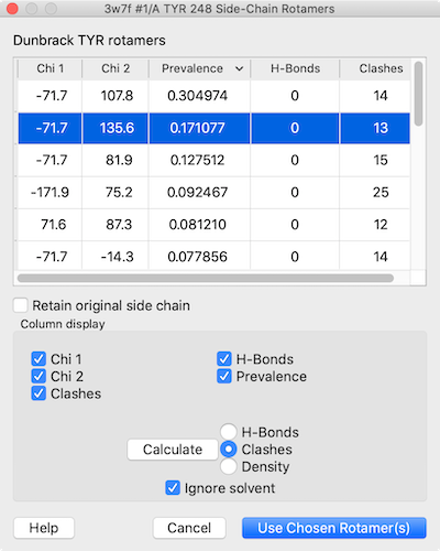
Via GUI: Select your target residue on the 3D structure. Then, go to Tools → Structure Editing → Rotamers. A specialized dialog window will pop up allowing you to select the new amino acid type. It will overlay the possible sidechain orientations (rotamers) ranked by library probability, allowing you to pick the one that best avoids steric clashes!

(Note: While there is a swapaa icon on the Right Mouse toolbar, it performs a "quick-swap" that blindly forces a default rotamer without opening a menu, so the structured Rotamers tool is highly preferred for accuracy).

Via Command Line: Let's mutate chain A's residue 243 to a neutral Alanine.

swapaa /A:243 ala

Tip

Check your Knockouts: If you mutate a polar residue to an Alanine and run the hbonds commands we learned back in Milestone 3, you will literally watch the dashed interaction lines vanish from the graphical display as the connection is broken!

4.5 Exporting the Prepared Structure

Once your protein is perfectly desolvated, cleaned of alt-locs, protonated, and mutated, it's time to export it. The .PDB format is the universal standard—ensuring you can port your prepared file perfectly into Maestro, AutoDock, PyMOL, or GROMACS.

Via GUI: Go to File → Save... and ensure the format drop-down is set to PDB or CIF.

Via Command Line:

save my_cleaned_protein.pdb format pdb

4.6 Python Showcase: The Automated Prep Pipeline

When processing tens or hundreds of structures, bioinformaticians rarely click menus. They script the entire cleanup process into an automated pipeline!

Open your Python Shell (Tools → General → Shell) and run:

from chimerax.core.commands import run

# Let's say you just loaded a raw PDB. We can clean it sequentially and instantly:
_ = run(session, 'delete solvent')
_ = run(session, 'altlocs clean')
_ = run(session, 'addh')
_ = run(session, 'save cleaned_target.pdb format pdb')

print("Automated Preparation Complete!")

(These targeted Python snippets will all be combined into a master automated pipeline script at the very end of the Walkthrough!)

---

Milestone 5: Advanced Features (MatchMaker, Morphing, and Movies)

While the previous structural milestones focused on preparing and analyzing static baseline targets, structural biology is highly dynamic. In this final showcase milestone, we will learn how to align homologous states, animate biological transitions, and aggregate everything into an automated python pipeline!

5.1 Structural Superimposition (MatchMaker)

Rather than digging into deep sequence-alignment theory here (which will be extensively covered later in your bioinformatics course), let's simply showcase how structurally powerful the ChimeraX engine is. We will load a classic homologous pair of a protein undergoing a massive active-site shift—Adenylate Kinase—in both its "Open" Apo state (4ake) and its "Closed" Holo state (1ake), and align them dynamically in 3D space.

Via GUI: First, open both structures. Then, go to Tools → Structure Analysis → Matchmaker. Choose your Reference structure to keep stationary (e.g., #1) and the structure you want to match to it (e.g., #2). Hit Apply.

Via Command Line:

# Open two distinct conformations of a homologous protein
open 4ake
open 1ake

# Align structure 2 onto structure 1 using their sequence homology
matchmaker #2 to #1

Info

Interpreting the MatchMaker Log: When you execute MatchMaker, ChimeraX outputs a massive analytical block to your Log. What does it actually mean? - Alignment parameters (Needleman-Wunsch & BLOSUM-62): Before matching the 3D structures, ChimeraX mathematically aligns their 1D amino acid sequences to map out which residues correspond to each other. - RMSD (Root-Mean-Square Deviation): The final output shows you the average distance (in Angstroms) between the aligned atoms. For 1ake vs 4ake, the RMSD over the "pruned" core is 1.083 Å (showing the stable backbone didn't move). However, the RMSD across all pairs is 8.240 Å! This huge difference proves that a massive, distinct conformational change occurred in the non-core regions (like the active site clamping shut).

5.2 Generating Conformational Trajectories (Morphing)

Now that the open and closed states are perfectly superimposed, wouldn't it be incredible to watch the active site physically snap shut? The morph command calculates the mathematical interpolation between the two structures.

(By applying the style stick and hbonds features from Milestone 3 onto this morph, you could literally watch a binding pocket dynamically clamp down on a ligand model!)

Via Command Line: (Note: Morphing is computationally dense and is exclusively initiated via the CLI).

# Generate a trajectory of 60 frames smoothly transitioning from structure 1 to 2
morph #1,2 frames 60

# Hide the original static models so we only see the moving trajectory (now model #3)
hide #1,2 models

Tip

A graphical Trajectory Slider panel will automatically pop up at the bottom of your screen! You can hit the Play button or drag the slider manually to scrub back and forth through the conformational change.

5.3 Directing Cinematic Movies

To present this moving morph trajectory in a seminar or lab meeting, we can record the graphics window straight to an .mp4 video. We will keep this concise—combining a spinning physical camera and the playback of the morph trajectory we just made.

Via GUI: You can manually record the screen by clicking the Record Video button (the classic video camera icon) located in the Home tab of the top ribbon toolbar.

Via Command Line: This is the classic, highly-controlled cinema recording sequence. Try copying and pasting this entire block:

# Start the camera recorder
movie record

# Play the morph sequence (assuming your morph trajectory is model #3)
coordset #3 1,60

# Add a slow 360-degree y-axis spin that spans 120 frames
turn y 3 120

# Wait 120 frames for the animation to finish calculating before cutting the camera
wait 120

# Render and compress the final mp4 to your computer
movie encode final_animation.mp4

5.4 The Capstone Python Showcase: The Automated Pipeline

Throughout this walkthrough, you have executed precise spatial operations step-by-step. But bioinformaticians don't click menus hundreds of times to prepare a massive virtual screening library—they use the ChimeraX Python API to stack all these skills into a single autonomous pipeline!

Here is the grand finale: a master helper script combining the exact commands you painstakingly learned in Milestones 1 through 4. It will fetch a structure, clean it, add hydrogens, render it, calculate a docking bounding-box, style the ligand, and save the artifact—completely autonomously.

Open your Python Shell (Tools → General → Shell) and run:

from chimerax.core.commands import run

print("Initiating Pipeline...")

# 1. Fetch the target and visualize it (Milestone 1 & 2)
run(session, 'open 1stp')
run(session, 'preset sil') # Applies "publication 1" silhouette preset

# 2. Structure Cleanup utilizing the All-In-One Dock Prep (Milestone 4)
run(session, 'altlocs clean')
run(session, 'dockprep')

# 3. Target the Binding Pocket (Ligand + 4 Angstroms) (Milestone 3)
run(session, 'show ligand')
run(session, 'show ligand :< 4')
run(session, 'style sel stick')
run(session, 'color sel byhetero')

# 4. Show Polar Interactions (Milestone 3)
run(session, 'hbonds ligand restrict protein color green')

# 5. Measure Docking Volume and Frame (Milestone 3/4)
run(session, 'molmap ligand 3 edgePadding 10')
run(session, 'volume #2 showOutlineBox true outlineBoxRgb cyan')
run(session, 'transparency #2 100')

# 6. Save the prepared image and final coordinates!
run(session, 'view ligand')
run(session, 'save Final_Docking_Prep.png width 1920 height 1080')
run(session, 'save Final_Prepared_Protein.pdb format pdb')

print("Automated Preparation Pipeline Executed Successfully! Pocket is ready for Docking.")

Congratulations! You have completed the ChimeraX Walkthrough. You now possess the dual GUI/CLI skillset required to physically meticulously dismantle, graphically analyze, and programmatically automate structural biochemistry targets.